9-5: Simulation (built-in) 9-5-3: ALS Concepts

The user should be aware that the ALS simulator translates the circuit into VHDL, then compiles the VHDL into a netlist for simulation. This means that when a layout or schematic is simulated, two new views of that cell are created: {VHDL} and {net.als}. Use the Edit VHDL View (in menu View) to see the VHDL code.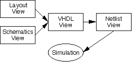

When simulation is requested, the cell in the current window is simulated. Date checking is performed to determine whether VHDL translation or netlist compilation is necessary. If you are currently editing a VHDL cell, it will not be regenerated from layout, even if the layout is more recent. Similarly, if you are currently editing a netlist cell, it will not be regenerated from VHDL, even if that VHDL is more recent. Thus, simulation of the currently edited cell is guaranteed.

Note that the presence of VHDL in the path to simulation means that it can simulate VHDL that is entered manually. You can type this VHDL directly into the cell (see Section 4-9 for more on text editing). Also, you can explicitly request that VHDL be produced from schematics or layout with the Make VHDL View command (in menu View).

This complete VHDL capability, combined with the Silicon Compiler which places and routes from VHDL descriptions, gives Electric a powerful facility for creating, testing, and constructing complex circuits from high-level specifications. See Section 9-12 for more on the Silicon Compiler.

Behavioral Models

When the VHDL for a circuit is compiled into a netlist, both connectivity and behavior are included. This is because the netlist format is hierarchical, and at the bottom of the hierarchy are behavioral primitives. Electric knows the behavioral primitives for MOS transistors, AND, OR, NAND, NOR, Inverter, and XOR gates. Other primitives can be defined by the user, and all of the existing primitives can be redefined.

To create (or redefine) a primitive's behavior, simply create the {net.als} view of the cell with that primitive's name. Use the New Cell... command (in menu Cell) and select the "netlist.als" view. For example, to define the behavior of an ALU cell, edit "alu{net.als}", and to redefine the behavior of a two-input And gate, edit "and2{net.als}". The compiler copies these textual cells into the netlist description whenever that node is referenced in the VHDL.

The netlist format provides three different types of entities: model, gate, and function. The model entity describes interconnectivity between other entities. It describes the hierarchy and the topology. The gate and function entities are at the primitive level. The gate uses a truth-table and the function makes reference to Java-coded behavior (which must be compiled into Electric, see the module "com.sun.electric.tool.simulation.als.UserCom.java"). Both primitive entities also allow the specification of operational parameters such as switching speed, capacitive loading and propagation delay. (The simulator determines the capacitive load, and thus the event switching delay, of each node of the system by considering the capacitive load of each primitive connected to a node as well as taking into account feedback paths to the node.)

A sample netlist describing an RS latch model is shown below. Note that the "#" character starts a comment.

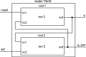# model declaration for the figure model main(set, reset, q, q_bar) inst1: nor2(reset, q_bar, q) inst2: nor2(q, set, q_bar) # gate description of nor2 gate nor2(in1, in2, out) t: delta=4.5e-9 + linear=5.0e-10 i: in1=L in2=L o: out=H@2 i: in1=H o: out=L@2 i: in2=H o: out=L@2 i: o: out=X@2

When combined, these entities represent a complete description of the circuit. Note that when a gate, function, or other model is referenced within a model description, there is a one-to-one correspondence between the signal names listed at the calling site and the signal names contained in the header of the called entity.

Simulator Internals

The ALS simulator simulates a set of simulation nodes. A simulation node is a connection point which may have one or more signals associated with it.

A simulation node can have 3 values (L, H, or X) and can have 4 strengths (off, node, gate, and VDD, in order of increasing strength). It is thus a 12-state simulator. In deciding the state of a simulation node at a particular time of the simulation, the simulator considers the states and strengths of all inputs driving the node.

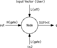Driving inputs may be from other simulation nodes, in which case the driving strength is "gate" (i.e. H(gate) indicates a logic HIGH state with gate driving strength), from a power or ground supply ("VDD" strength) or from the user (any strength). If no user vector has been input at the current simulation time, then the input defaults to the "off" strength.

In the above example, the combination of a high and a low driving input at the same strength from the signals "out" and "in2" result in the simulation algorithm assigning the X (undefined) state to the output signal represented by "q". This example also shows the behavior of part of the simulation engine's arbitration algorithm, which dictates that an undefined state exists if a simulator node is being driven by signals with the same strength but different states, providing that the strength of the driving signals in conflict is the highest state driving the node.

Another important concept for the user to remember is that the simulator is an event-driven simulator. When a simulation node changes state, the simulation engine looks through the netlist for other nodes that could potentially change state. Obviously, only simulation nodes joined by model, gate or function entities can potentially change state. If a state change, or event, is required (based on the definition of the inter-nodal behavior as given by the model, gate or function definition), the event is added to the list of events scheduled to occur later in the simulation. When the event time is reached and the event is fired, the simulator must again search the database for other simulation nodes which may potentially change state. This process continues until it has propagated across all possible nodes and events.

Previous

Table of Contents

Next