 |
9-4: Simulation |
|
|
9-4: Simulation |
|
The Simulation (SPICE), Simulation (Verilog), and Simulation (Others) commands of the Tools menu are able to produce input specifications for a number of different simulators. All these commands work on the current cell and require that all named points be exports. It is also necessary to have power and ground exports.
The possible simulators include circuit-level (SPICE, Maxwell), switch-level (IRSIM, ESIM, RSIM, RNL, COSMOS, and MOSSIM), gate-level (ABEL-PAL), and functional (VERILOG, TEGAS, and SILOS). In addition, you can generate a deck for the FastHenry inductance analysis system.
To produce an input deck for any of these simulators, use the Write XXX Deck command (where XXX is the simulator's name). In addition to these simulators, an EDIF netlist can be produced with the EDIF (Electronic Design Interchange Format) subcommand of the Export command of the File menu.
Besides generating Verilog decks, it is possible to annotate circuits with additional Verilog declarations and code that will be included in the deck. The subcommands Add Verilog Code and Add Verilog Declaration of the Simulation (Verilog) command of the Tools menu allow you to click in the circuit and type code or declarations. These pieces of text can be manipulated like any other text object (see Section 6-8 on text).
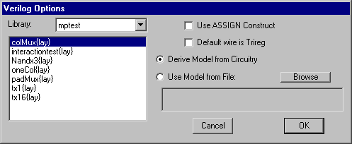
Additional control of Verilog deck generation is accomplished with the Verilog Options... subcommand. A checkbox lets you choose whether or not to use the Verilog "assign" construct. You can control the type of Verilog declaration that will be used for wires ("wire" by default, "trireg" if checked). Note that this can be overridden with the Set Verilog Wire subcommand of the Simulation (Verilog) command of the Tools menu.
The Verilog Options dialog also lets you attach disk files with Verilog code to any cell in the library. Once attached, the generated Verilog will use the contents of that file instead of examining the cell contents. This allows you to create your own definitions in situations where the derived Verilog would be too complex or otherwise incorrect. For an example of Verilog layout and code, look at the cell "tool-SimulateVERILOG" in the library "samples.txt" (you can read the library with the Readable Dump subcommand of the Import command of the File menu).
After running a Verilog simulation, you can read the dump file into Electric and display it in a waveform window. This is done with the Plot Verilog VCD Dump... subcommand of the Simulation (Verilog) command of the Tools menu (or just Plot Verilog for This Cell if the cell name and file name are the same). Control of the waveform window is described more fully in Section 10-2.
SPICE circuit simulation is a special case in Electric. Because the simulator is not interactive, all specifications must be done graphically, in advance. Note that the example shown here is available in the "samples.txt" library as cell "tool-SimulateSPICE" (you can read the library with the Readable Dump subcommand of the Import command of the File menu).
| All input values to SPICE are controlled with special nodes, found in the New SPICE Part command of the Edit menu. These parts are also available from the "Spice" button in the component menu of the Schematics technologies. Note that the first time any SPICE node is placed, the library of SPICE parts is loaded into Electric. | 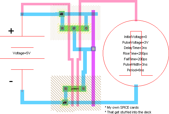 |
The SPICE primitives described here are for Electric's default set. However, additional sets can (and have) been written. To choose another set, change the "SPICE primitive set" popup in the SPICE Options... subcommand of the Simulation (SPICE) command of the Tools menu.
In this example, there is a 5-volt supply on the left. It was created by using the DC Voltage Source subcommand. Once placed, the text that reads "Voltage=0V" is selected and modified (either with Get Info or by double-clicking on it). The Pulse input signal on the right is created with the Pulse subcommand (it has 7 parameters).
This example also shows the ability to add arbitrary text to the SPICE deck with the Add SPICE Card subcommand of the Simulation (SPICE) command of the Tools menu. The command creates a piece of text (shown in the lower-right) that can be modified arbitrarily.
There are both voltage and current sources, in AC and DC form. The pulse input sources are available as voltage and current. A set of "two-gate" devices are also available: CCCS, CCVS, VCCS, VCVS, and Transmission.
It is possible to specify Transient, DC, or AC analysis by using the Transient Analysis, DC Analysis, and AC Analysis subcommands. Only one such element may exist in a circuit.
Bipolar transistors have their substrate connected to ground by default. If a Substrate node is encountered, its network will be used for the substrate connection of these transistors instead. The Well subcommand can be used to specify the well network.
For advanced users, there are two special SPICE nodes: Node Set and Extension. The Node Set may be parameterized with an arbitrary piece of SPICE code. Truly advanced users may create their own SPICE nodes by modifying the cells in the SPICE library.
Another option that can be used when modeling transistors and other component is to set a specific SPICE model to use for that component. Use the Set Spice Model... subcommand of the Simulation (SPICE) command of the Tools menu to create a SPICE model field on the selected component. Then you can select that text and set it.
The Add Multiplier subcommand places a multiplier on the currently selected node. Multipliers (also called "M" factors) scale the size of transistors inside of them.
 |
Some nongraphical information can also be given to the SPICE simulator with the SPICE Options...
subcommand of the Simulation (SPICE) command of the Tools menu.
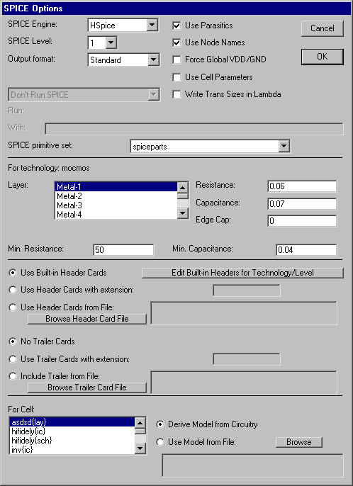
The top part of this dialog allows you to control many of the SPICE deck parameters such as the SPICE format (SPICE 2, SPICE 3, HSPICE, PSPICE, Gnucap, or SmartSPICE), the SPICE level (1, 2, or 3), what format to expect when reading SPICE output, whether to use parasitics in the deck, whether to use actual node names in the deck (SPICE 2 cannot handle this), and whether to force power and ground to be global signal names. |
When "Use Cell Parameters" is checked, any parameters defined on the cell will appear in the SPICE deck. When this is not checked, each parameterized cell appears multiple times in the deck, once for each different parameter combination. See Section 6-8 for more on parameters.
The "Write Trans Sizes in Lambda" dialog requests that the SPICE deck contain scalable size information instead of absolute size information.
UNIX systems can choose to run SPICE after the deck has been generated. In addition, they can specify special command-line options to be given to SPICE (the "With" field). There are five options:
The middle section of the Spice Options dialog controls technology-specific information. The upper-middle section controls parasitics, including per-layer resistance, capacitance, and edge-capacitance. You can also set the minimum resistance and capacitance for the entire technology. The lower-middle section controls header cards (placed at the start of the SPICE deck) and trailer cards (placed at the end of the SPICE deck). This dialog allows you to specify a disk file with header cards or trailer cards to be used instead of the built-in set. You can specify a particular file or request that the system search for files with the cell's name and a given extension. You can also edit the built-in header cards for the current technology by using the "Edit Built-in Header Cards" button, which invokes an editing window (see Section 4-10 for more on text editing).
Note that the header, trailer, and parasitic information is specific to a particular technology. If you set this information for one technology, but then use another technology when generating the SPICE deck, the information that you set will not be used. Note also that schematics, although a technology in Electric, are not considered to be SPICE technology. You can set the proper layout technology that you want to use when dealing with schematics by using the Technology Options command of the Technology menu and setting the "Use Lambda values from this Technology" popup.
The bottom section of the dialog allows you to specify a disk file of SPICE cards that will be used to describe any cell. This disk file replaces the any SPICE description that may be derived from the circuitry.
Electric has a set of SPICE elements (DC Voltage Source, CCCS, Pulse, etc.) that create appropriate SPICE deck cards. These elements are found in the readable dump file "spiceparts.txt" in the "lib" directory. This library consists of a set of icon cells that describe the various SPICE primitives, and each icon has a special Spice Template that describes the SPICE card to generate.
Users can define their own SPICE elements by creating new icons in this or a new library. The icon must have graphics, exports, parameters, and a template. Parameters are created with the Cell Parameters... subcommand of the Attributes command of the Info menu (see Section 6-8 for more on parameters). The SPICE template is created with the Set Generic SPICE Template subcommand of the Simulation (SPICE) command of the Tools menu. If the template is specific to a particular version of SPICE, use the appropriate template subcommand (Set SPICE 2 Template, Set SPICE 3 Template, Set HSPICE Template, Set PSPICE Template, Set GnuCAP Template, or Set SmartSPICE Template).
You can also create Verilog elements by using the Set Verilog Template subcommand of the Simulation (Verilog) command of the Tools menu. This template has the format as illustrated below. Note that a single cell can contain both Verilog and multiple SPICE templates.
The DC Voltage Source primitive is illustrated here.
Graphics is placed to describe the look of the symbol (a "battery" look).
Exports are created at the top and bottom of the battery with the names "plus" and "minus".
A single parameter is defined called "Voltage" with a default value of "0V".
Finally, a SPICE template is created that has the string
V$(node_name) $(plus) $(minus) DC $(Voltage) | 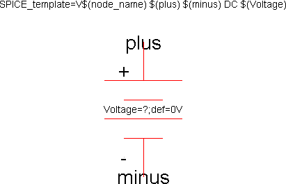 |
This string contains substitution expressions of the form $(SOMETHING)
where SOMETHING can be an export name, a variable, or "node_name".
So, in this example, $(node_name) will be replaced with the name of the voltage node;
$(plus) will be replaced with the net name attached to the positive terminal;
and $(Voltage) will be replaced with the voltage value specified by the user.
The set of SPICE primitives in Electric is useful, but far from complete. A second set, called "SpicePartsS3", is tailored towards special SPICE3 primitives. There are no Verilog primitives in the current release of Electric. Users who define new primitives are encouraged to share these with the entire community by contacting Static Free Software.
Once SPICE has been run, you can see a plot of the simulation by reading the SPICE output file back into Electric. Since there are may formats of SPICE output, you must first set the "SPICE Engine" and the "Output format" fields of the SPICE Options... dialog. The "Output format" field can be "Standard" for the default output of the SPICE engine; "Raw" for rawfile dumps; and "Raw/Smart" for the rawfile dumps from SmartSPICE.
When Electric knows what type of SPICE output file to expect, use the Plot SPICE Listing... command to read the file (or just Plot Spice for This Cell if the cell name and file name are the same). The waveforms will appear in a window:
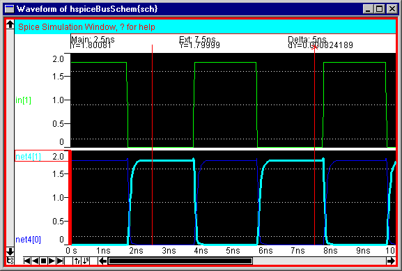
The waveform window is tied to an associated schematics or layout window. Clicking on a signal in the waveform windows highlights the equivalent circuitry in the other window, and clicking on an arc in the schematics or layout window causes the waveform signal to be selected. Both the waveform window and the associated schematics/layout window are highlighted with a red border to indicate that they are part of the simulation activity.
The horizontal axis of the simulation window shows time. Two vertical lines are drawn, called the "main" and the "extension" cursors (the extension cursor has an "X" drawn at its top). You can click over these cursors and drag them to different time locations. The location of the cursors, and the value of the selected signal at those times, is shown at the top. The time axis can also be controlled with the appropriate Windows menu commands. Use Zoom Out and Zoom In to scale the time axis by a factor of two. Use Fill Window to display the entire range of data, fit to the screen. Use Focus on Highlighted to display the range between the main and extension cursors.
You can control which signals are displayed in the waveform window. To remove a signal, select its name and type "r" or the DELETE key. When adding a signal, you have a choice of showing it overlaid with an existing signal, or in its own graph. Typing "o" causes the signal to be overlaid onto the currently selected signal, and typing "a" causes the signal to be added in its own "frame". If you type "o" or "a" into the waveform window, you will be prompted for a list of signal names to display. If you type "o" or "a" in the assiciated schematics/layout window, then the selected signal from that window will be added to the waveform display.
Besides the time axis, it is possible to zoom and pan the vertical axis of a frame of the waveform window. Typing '7' doubles the scale (zooms-in) and typing '0' halves the scale (zooms-out). Type '9' to restore the scale so that the data fills the screen. Use '8' and '2' to shift the data values up and down.
One final feature is the ability to take a snapshot of the waveform window. Typing "p" preserves the waveform in the database (a cell with the "simulation-snapshot" view is created with artwork components).
Here is a summary of the single-key commands available in SPICE windows:
| Add signal | Add selected network to waveform window | |
| Overlay signal on top of currently selected signal line | Overlay selected network on top of currently selected signal line | |
DEL | Remove selected signal | |
| Zoom in vertically (double data scale) | ||
| Zoom out vertically (halve data scale) | ||
| Scale data to fill the display | ||
| Shift data up by 1/4 screen | ||
| Shift data down by 1/4 screen | ||
| Preserve snapshot of waveform window | ||
| Move down the hierarchy (into the selected cell) | ||
| Move up the hierarchy (out of the current cell) | ||
| Print this listing of single-key commands | Print this listing of single-key commands |
FastHenry is an inductance analysis tool (see the papers of Jacob White). When a FastHenry deck is generated, a subset of the arcs in the current cell are written. To include an arc in the FastHenry deck, select it and use the FastHenry Arc Info... subcommand of the Simulation (Others) command of the Tools menu.
| This command presents a dialog with FastHenry factors for the selected arc. The most important factor is in the upper-left: "Include this arc in FastHenry analysis". By checking this, the arc is described in the FastHenry deck. Once this is checked, other fields in the dialog become active. You can set the thickness of this arc (the default value shown will be used if no override is specified). You can set the number of subdivisions that will be used in height and width (again, defaults are shown). You can even set the height of the two ends of the arc. | 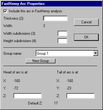 |
After all arcs have been marked, you can generate a FastHenry deck with the Write FastHenry Deck... subcommand of the Simulation (Others) command of the Tools menu. Before doing that, however, you can set other options for FastHenry deck generation To do this, use the FastHenry Options... subcommand of the Simulation (Others) command of the Tools menu.
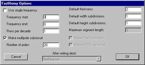
This dialog allows you to set the type of frequency analysis (single frequency or a sequence specified by a start, end, and number of runs per frequency). You can choose to use single or multiple-pole analysis (and if multiple, you can specify the number of poles). The FastHenry Options dialog also allows you to set defaults for the individual arcs that will be included in the deck. You can specify the default thickness, and the default number of subdivisions (in height and width). Other options are not implemented at this time.
 |
Previous |  |
Table of Contents | Next |  |